Temporal
This package provides a flexible & efficient time series class, TS, for the Julia programming language. While still early in development, the overarching goal is for the class to be able to slice & dice data with the rapid prototyping speed of R's xts and Python's pandas packages, while retaining the performance one expects from Julia.
Installation
Temporal can be easily installed using Julia's built-in package manager.
using Pkg
Pkg.add("Temporal")
using Temporal
Introduction
The TS Type
Member Variables
TS objects store three member variables to facilitate data manipulation and analysis.
values: anArrayof the values of the time series dataindex: aVectorwhose elements are either of typeDateorDateTimeindexing the values of the time seriesfields: aVectorwhose elements are of typeSymbolrepresenting the column names of the time series data
Constructors
The TS object type can be created in a number of ways. One thing to note is that when constructing the TS object, passing only the Array of values will automatically create the index and the fields members. When not passed explicitly, the index defaults to a series of dates that ends with today's date, and begins N-1 days before (where N is the number of rows of the values). The fields (or column names) are automatically set in a similar fashion as Excel when not given explicitly (A, B, C, ..., X, Y, Z, AA, AB, ...).
julia> using Temporal, Dates

julia> N, K = 100, 4;

julia> Random.seed!(1);
ERROR: UndefVarError: Random not defined

julia> values = rand(N, K);

julia> TS(values)
100x4 TS{Float64,Dates.Date}: 2019-10-15 to 2020-01-22

Index       A       B       C       D
2019-10-15  0.2177  0.5643  0.7495  0.6068
2019-10-16  0.2423  0.2202  0.5364  0.4645
2019-10-17  0.2919  0.3229  0.9707  0.8092
2019-10-18  0.2403  0.6756  0.9316  0.172
2019-10-19  0.9082  0.8792  0.2063  0.2342
2019-10-20  0.6194  0.4831  0.2652  0.5802
2019-10-21  0.6887  0.6364  0.449   0.1051
⋮
2020-01-15  0.6132  0.2045  0.1095  0.7481
2020-01-16  0.0341  0.8973  0.4979  0.9655
2020-01-17  0.6647  0.2151  0.6944  0.2312
2020-01-18  0.0892  0.7273  0.0243  0.2069
2020-01-19  0.8108  0.6423  0.197   0.1179
2020-01-20  0.1057  0.627   0.5414  0.5552
2020-01-21  0.5531  0.9182  0.8844  0.9071
2020-01-22  0.7044  0.9542  0.5507  0.9445

julia> index = today()-Day(N-1):Day(1):today();

julia> TS(values, index)
100x4 TS{Float64,Dates.Date}: 2019-10-15 to 2020-01-22

Index       A       B       C       D
2019-10-15  0.2177  0.5643  0.7495  0.6068
2019-10-16  0.2423  0.2202  0.5364  0.4645
2019-10-17  0.2919  0.3229  0.9707  0.8092
2019-10-18  0.2403  0.6756  0.9316  0.172
2019-10-19  0.9082  0.8792  0.2063  0.2342
2019-10-20  0.6194  0.4831  0.2652  0.5802
2019-10-21  0.6887  0.6364  0.449   0.1051
⋮
2020-01-15  0.6132  0.2045  0.1095  0.7481
2020-01-16  0.0341  0.8973  0.4979  0.9655
2020-01-17  0.6647  0.2151  0.6944  0.2312
2020-01-18  0.0892  0.7273  0.0243  0.2069
2020-01-19  0.8108  0.6423  0.197   0.1179
2020-01-20  0.1057  0.627   0.5414  0.5552
2020-01-21  0.5531  0.9182  0.8844  0.9071
2020-01-22  0.7044  0.9542  0.5507  0.9445

julia> fields = [:A, :B, :C, :D];

julia> X = TS(values, index, fields)
100x4 TS{Float64,Dates.Date}: 2019-10-15 to 2020-01-22

Index       A       B       C       D
2019-10-15  0.2177  0.5643  0.7495  0.6068
2019-10-16  0.2423  0.2202  0.5364  0.4645
2019-10-17  0.2919  0.3229  0.9707  0.8092
2019-10-18  0.2403  0.6756  0.9316  0.172
2019-10-19  0.9082  0.8792  0.2063  0.2342
2019-10-20  0.6194  0.4831  0.2652  0.5802
2019-10-21  0.6887  0.6364  0.449   0.1051
⋮
2020-01-15  0.6132  0.2045  0.1095  0.7481
2020-01-16  0.0341  0.8973  0.4979  0.9655
2020-01-17  0.6647  0.2151  0.6944  0.2312
2020-01-18  0.0892  0.7273  0.0243  0.2069
2020-01-19  0.8108  0.6423  0.197   0.1179
2020-01-20  0.1057  0.627   0.5414  0.5552
2020-01-21  0.5531  0.9182  0.8844  0.9071
2020-01-22  0.7044  0.9542  0.5507  0.9445
Equivalently, one can construct a TS object using the standard rand construction approach.
julia> Random.seed!(1);
ERROR: UndefVarError: Random not defined

julia> Y = rand(TS, (N,K))
100x4 TS{Float64,Dates.Date}: 2019-10-15 to 2020-01-22

Index       A       B       C       D
2019-10-15  0.7602  0.0188  0.5162  0.0155
2019-10-16  0.8095  0.238   0.9634  0.8136
2019-10-17  0.4684  0.8535  0.3422  0.3003
2019-10-18  0.9588  0.5026  0.6863  0.2596
2019-10-19  0.9123  0.4947  0.771   0.0745
2019-10-20  0.3779  0.1386  0.7488  0.0147
2019-10-21  0.2779  0.7322  0.8518  0.8784
⋮
2020-01-15  0.8992  0.8452  0.1165  0.0461
2020-01-16  0.1477  0.1004  0.238   0.2677
2020-01-17  0.4336  0.2912  0.5884  0.4724
2020-01-18  0.3302  0.2351  0.6646  0.7083
2020-01-19  0.1032  0.3069  0.0261  0.243
2020-01-20  0.0414  0.4943  0.7607  0.5045
2020-01-21  0.8222  0.5318  0.6282  0.9256
2020-01-22  0.035   0.2935  0.6676  0.9736

julia> X == Y
false
Operations
The standard operations that apply to Array objects will generally also work for TS objects. (If there is an operation that does not have a method defined for the TS type that you feel is missing, please don't hesitate to submit an issue and we will get it added ASAP.)
julia> cumsum(X)
100x4 TS{Float64,Dates.Date}: 2019-10-15 to 2020-01-22

Index       A        B        C        D
2019-10-15  0.2177   0.5643   0.7495   0.6068
2019-10-16  0.46     0.7844   1.2859   1.0713
2019-10-17  0.7519   1.1073   2.2566   1.8805
2019-10-18  0.9922   1.7829   3.1882   2.0526
2019-10-19  1.9004   2.6621   3.3946   2.2868
2019-10-20  2.5198   3.1451   3.6598   2.867
2019-10-21  3.2085   3.7815   4.1088   2.9721
⋮
2020-01-15  42.6786  46.3207  41.0402  43.1286
2020-01-16  42.7128  47.218   41.5381  44.0941
2020-01-17  43.3774  47.4332  42.2325  44.3253
2020-01-18  43.4666  48.1604  42.2568  44.5321
2020-01-19  44.2774  48.8027  42.4538  44.65
2020-01-20  44.383   49.4297  42.9952  45.2052
2020-01-21  44.9361  50.348   43.8796  46.1123
2020-01-22  45.6406  51.3022  44.4302  47.0568

julia> cumprod(1 + diff(log(Y)))
ERROR: MethodError: no method matching log(::TS{Float64,Dates.Date})
Closest candidates are:
  log(!Matched::Float16) at math.jl:1019
  log(!Matched::Complex{Float16}) at math.jl:1020
  log(!Matched::Float64) at special/log.jl:254
  ...

julia> X + Y
100x4 TS{Float64,Dates.Date}: 2019-10-15 to 2020-01-22

Index       A       B       C       D
2019-10-15  0.9779  0.5831  1.2657  0.6223
2019-10-16  1.0518  0.4582  1.4998  1.2781
2019-10-17  0.7603  1.1764  1.3129  1.1095
2019-10-18  1.1991  1.1782  1.6179  0.4316
2019-10-19  1.8206  1.3739  0.9773  0.3087
2019-10-20  0.9973  0.6217  1.014   0.5949
2019-10-21  0.9665  1.3686  1.3008  0.9835
⋮
2020-01-15  1.5124  1.0497  0.2259  0.7943
2020-01-16  0.1819  0.9977  0.736   1.2332
2020-01-17  1.0983  0.5063  1.2828  0.7036
2020-01-18  0.4193  0.9623  0.6889  0.9151
2020-01-19  0.914   0.9491  0.2231  0.3609
2020-01-20  0.1471  1.1213  1.3022  1.0597
2020-01-21  1.3752  1.45    1.5126  1.8327
2020-01-22  0.7394  1.2477  1.2183  1.9181

julia> abs.(sin.(X))
100x4 TS{Float64,Dates.Date}: 2019-10-15 to 2020-01-22

Index       A       B       C       D
2019-10-15  0.216   0.5348  0.6813  0.5703
2019-10-16  0.24    0.2184  0.5111  0.448
2019-10-17  0.2878  0.3173  0.8253  0.7238
2019-10-18  0.238   0.6254  0.8026  0.1712
2019-10-19  0.7884  0.7702  0.2049  0.2321
2019-10-20  0.5806  0.4645  0.2621  0.5482
2019-10-21  0.6355  0.5943  0.4341  0.1049
⋮
2020-01-15  0.5755  0.2031  0.1092  0.6803
2020-01-16  0.0341  0.7816  0.4776  0.8223
2020-01-17  0.6168  0.2135  0.6399  0.2291
2020-01-18  0.089   0.6648  0.0243  0.2054
2020-01-19  0.7248  0.599   0.1957  0.1176
2020-01-20  0.1055  0.5868  0.5154  0.5271
2020-01-21  0.5253  0.7945  0.7735  0.7877
2020-01-22  0.6476  0.8159  0.5232  0.8102
Usage
Data Input/Output
There are currently several options for how to get time series data into the Julia environment as Temporal.TS objects.
- Data Vendor Downloads
- Local Flat Files (CSV, TSV, etc.)
Quandl Data Downloads
julia> corn = quandl("CHRIS/CME_C1", from="2010-06-09", thru=string(Dates.today()), freq='w')  # weekly corn price history
503x8 TS{Float64,Dates.Date}: 2010-06-13 to 2020-01-26

Index       Open    High    Low     Last    Change  Settle  Volume    Previous Day Open Interest
2010-06-13  345.5   349.75  345.25  349.5   NaN     349.5   161773.0  353285.0
2010-06-20  357.0   364.0   356.5   360.75  NaN     360.75  101835.0  262392.0
2010-06-27  345.0   345.25  339.0   340.5   NaN     340.5   125609.0  159949.0
2010-07-04  362.5   365.75  361.25  364.0   NaN     364.0   17351.0   20723.0
2010-07-11  377.5   377.5   374.0   375.25  NaN     375.25  7471.0    5603.0
2010-07-18  391.0   395.5   387.75  394.75  NaN     394.75  87390.0   400595.0
2010-07-25  377.0   377.5   370.0   371.25  NaN     371.25  68229.0   401677.0
⋮
2019-12-08  364.75  368.75  364.75  366.5   1.0     366.5   960.0     2286.0
2019-12-15  373.75  374.5   366.25  366.25  0.75    366.25  88.0      165.0
2019-12-22  386.5   389.5   386.0   387.75  1.25    387.75  68692.0   754264.0
2019-12-29  388.0   391.0   388.0   390.0   1.5     390.0   73843.0   748797.0
2020-01-05  391.5   392.0   385.5   386.0   5.0     386.5   112048.0  740797.0
2020-01-12  383.25  386.75  376.5   385.75  2.5     385.75  206470.0  733377.0
2020-01-19  377.0   389.5   376.75  389.0   13.75   389.25  275953.0  745179.0
2020-01-26  389.0   389.25  384.25  387.5   1.75    387.5   168620.0  707498.0

julia> corn = dropnan(corn)  # remove rows with any NaN
310x8 TS{Float64,Dates.Date}: 2014-02-23 to 2020-01-26

Index       Open    High    Low     Last    Change  Settle  Volume    Previous Day Open Interest
2014-02-23  455.5   456.5   450.25  452.2   2.6     453.0   145346.0  244376.0
2014-03-02  448.0   458.75  447.75  458.0   9.4     457.5   37182.0   38695.0
2014-03-09  485.25  495.0   478.0   481.0   4.6     481.0   7141.0    7124.0
2014-03-16  484.5   484.75  480.5   485.2   1.0     472.25  316.0     515.0
2014-03-23  478.5   481.0   476.0   477.4   0.4     479.0   87347.0   548999.0
2014-03-30  491.0   496.25  489.0   490.0   7.4     492.0   120358.0  530465.0
2014-04-06  498.0   502.0   492.5   502.0   1.5     501.5   104110.0  482614.0
⋮
2019-12-08  364.75  368.75  364.75  366.5   1.0     366.5   960.0     2286.0
2019-12-15  373.75  374.5   366.25  366.25  0.75    366.25  88.0      165.0
2019-12-22  386.5   389.5   386.0   387.75  1.25    387.75  68692.0   754264.0
2019-12-29  388.0   391.0   388.0   390.0   1.5     390.0   73843.0   748797.0
2020-01-05  391.5   392.0   385.5   386.0   5.0     386.5   112048.0  740797.0
2020-01-12  383.25  386.75  376.5   385.75  2.5     385.75  206470.0  733377.0
2020-01-19  377.0   389.5   376.75  389.0   13.75   389.25  275953.0  745179.0
2020-01-26  389.0   389.25  384.25  387.5   1.75    387.5   168620.0  707498.0
Yahoo! Finance Downloads
julia> snapchat_prices = yahoo("SNAP", from="2017-03-03")  # historical prices for Snapchat since its IPO date
726x6 TS{Float64,Dates.Date}: 2017-03-03 to 2020-01-21

Index       Open    High    Low     Close  AdjClose  Volume
2017-03-03  26.39   29.44   26.06   27.09  27.09     1.481664e8
2017-03-06  28.17   28.25   23.77   23.77  23.77     7.2903e7
2017-03-07  22.21   22.5    20.64   21.44  21.44     7.18578e7
2017-03-08  22.03   23.43   21.31   22.81  22.81     4.98191e7
2017-03-09  23.17   23.68   22.51   22.71  22.71     2.58032e7
2017-03-10  23.36   23.4    22.0    22.07  22.07     1.83376e7
2017-03-13  22.05   22.15   20.96   21.09  21.09     2.06059e7
⋮
2020-01-09  17.29   17.93   17.04   17.36  17.36     6.27142e7
2020-01-10  17.66   17.73   17.28   17.41  17.41     2.56217e7
2020-01-13  17.48   18.0    17.3    18.0   18.0      2.23939e7
2020-01-14  17.99   18.09   17.665  17.99  17.99     2.53901e7
2020-01-15  18.0    18.52   17.97   18.19  18.19     2.33813e7
2020-01-16  18.02   18.41   17.777  18.25  18.25     2.70507e7
2020-01-17  19.1    19.29   18.76   19.11  19.11     4.63173e7
2020-01-21  19.02   19.25   18.77   19.0   19.0      2.47756e7

julia> exxon_dividends = yahoo("XOM", event="div", from="2000-01-01", thru="2009-12-31")  # all dividend payments Exxon disbursed during the 2000's
42x1 TS{Float64,Dates.Date}: 2000-02-09 to 2009-11-09

Index       Dividends
2000-02-09  0.44
2000-05-11  0.44
2000-08-10  0.44
2000-11-09  0.44
2001-02-07  0.44
2001-02-08  0.44
2001-05-10  0.44
⋮
2008-02-07  0.35
2008-05-09  0.4
2008-08-11  0.4
2008-11-07  0.4
2009-02-06  0.4
2009-05-11  0.42
2009-08-11  0.42
2009-11-09  0.42
Flat File I/O
julia> filepath = "tmp.csv"
"tmp.csv"

julia> tswrite(corn, filepath)

julia> tsread(filepath) == corn
true
Subsetting/Indexing
Easily one of the more important parts of handling time series data is the ability to retrieve from that time series specific portions of the data that you want. To this end, TS objects provide a fairly flexible indexing interface to make it easier to slice & dice data in the ways commonly desired, while maintaining an emphasis on speed and performance wherever possible.
As an example use case, let us analyze the price history of front-month crude oil futures.
julia> crude = quandl("CHRIS/CME_CL1")  # download crude oil prices from Quandl
9250x8 TS{Float64,Dates.Date}: 1983-03-30 to 2020-01-21

Index       Open    High    Low     Last    Change  Settle  Volume      Previous Day Open Interest
1983-03-30  29.01   29.56   29.01   29.4    NaN     29.4    949.0       470.0
1983-03-31  29.4    29.6    29.25   29.29   NaN     29.29   521.0       523.0
1983-04-04  29.3    29.7    29.29   29.44   NaN     29.44   156.0       583.0
1983-04-05  29.5    29.8    29.5    29.71   NaN     29.71   175.0       623.0
1983-04-06  29.9    29.92   29.65   29.9    NaN     29.9    392.0       640.0
1983-04-07  29.9    30.2    29.86   30.17   NaN     30.17   817.0       795.0
1983-04-08  30.65   30.65   30.25   30.38   NaN     30.38   365.0       651.0
⋮
2020-01-09  59.99   60.31   58.66   59.59   0.05    59.56   738556.0    321112.0
2020-01-10  59.61   59.78   58.85   59.12   0.52    59.04   579590.0    281957.0
2020-01-13  59.04   59.27   57.91   58.09   0.96    58.08   572099.0    235115.0
2020-01-14  58.03   58.72   57.72   58.14   0.15    58.23   494837.0    185715.0
2020-01-15  58.2    58.36   57.36   58.1    0.42    57.81   426110.0    136771.0
2020-01-16  58.1    58.87   57.56   58.59   0.71    58.52   178898.0    96523.0
2020-01-17  58.59   58.98   58.27   58.81   0.02    58.54   118984.0    73735.0
2020-01-21  59.17   59.73   57.68   58.25   0.2     58.34   36251.0     31495.0

julia> crude = dropnan(crude)  # remove the missing values from the downloaded data
1488x8 TS{Float64,Dates.Date}: 2014-02-18 to 2020-01-21

Index       Open    High    Low     Last    Change  Settle  Volume      Previous Day Open Interest
2014-02-18  100.32  103.25  100.23  102.43  2.13    102.43  168003.0    66485.0
2014-02-19  103.14  103.8   102.4   103.31  0.88    103.31  85672.0     29350.0
2014-02-20  103.41  103.5   102.75  103.05  0.39    102.92  36274.0     29350.0
2014-02-21  102.87  102.92  101.69  102.2   0.55    102.2   163793.0    320747.0
2014-02-24  102.29  103.45  101.97  102.82  0.62    102.82  169414.0    324685.0
2014-02-25  102.8   102.84  101.02  101.83  0.99    101.83  179081.0    320864.0
2014-02-26  102.04  102.9   101.58  102.55  0.76    102.59  187756.0    318599.0
⋮
2020-01-09  59.99   60.31   58.66   59.59   0.05    59.56   738556.0    321112.0
2020-01-10  59.61   59.78   58.85   59.12   0.52    59.04   579590.0    281957.0
2020-01-13  59.04   59.27   57.91   58.09   0.96    58.08   572099.0    235115.0
2020-01-14  58.03   58.72   57.72   58.14   0.15    58.23   494837.0    185715.0
2020-01-15  58.2    58.36   57.36   58.1    0.42    57.81   426110.0    136771.0
2020-01-16  58.1    58.87   57.56   58.59   0.71    58.52   178898.0    96523.0
2020-01-17  58.59   58.98   58.27   58.81   0.02    58.54   118984.0    73735.0
2020-01-21  59.17   59.73   57.68   58.25   0.2     58.34   36251.0     31495.0
Column Indexing
The fields member of the Temporal.TS object (wherein the column names are stored) are represented using Julia's builtin Symbol datatype.
julia> crude[:Settle]
1488x1 TS{Float64,Dates.Date}: 2014-02-18 to 2020-01-21

Index       Settle
2014-02-18  102.43
2014-02-19  103.31
2014-02-20  102.92
2014-02-21  102.2
2014-02-24  102.82
2014-02-25  101.83
2014-02-26  102.59
⋮
2020-01-09  59.56
2020-01-10  59.04
2020-01-13  58.08
2020-01-14  58.23
2020-01-15  57.81
2020-01-16  58.52
2020-01-17  58.54
2020-01-21  58.34

julia> crude[[:Settle,:Volume]]
1488x2 TS{Float64,Dates.Date}: 2014-02-18 to 2020-01-21

Index       Settle  Volume
2014-02-18  102.43  168003.0
2014-02-19  103.31  85672.0
2014-02-20  102.92  36274.0
2014-02-21  102.2   163793.0
2014-02-24  102.82  169414.0
2014-02-25  101.83  179081.0
2014-02-26  102.59  187756.0
⋮
2020-01-09  59.56   738556.0
2020-01-10  59.04   579590.0
2020-01-13  58.08   572099.0
2020-01-14  58.23   494837.0
2020-01-15  57.81   426110.0
2020-01-16  58.52   178898.0
2020-01-17  58.54   118984.0
2020-01-21  58.34   36251.0

julia> crude[1:100, :Volume]
100x1 TS{Float64,Dates.Date}: 2014-02-18 to 2014-07-10

Index       Volume
2014-02-18  168003.0
2014-02-19  85672.0
2014-02-20  36274.0
2014-02-21  163793.0
2014-02-24  169414.0
2014-02-25  179081.0
2014-02-26  187756.0
⋮
2014-06-30  229049.0
2014-07-01  231393.0
2014-07-02  249258.0
2014-07-03  185064.0
2014-07-07  170076.0
2014-07-08  249378.0
2014-07-09  265417.0
2014-07-10  253268.0
A series of financial extractor convenience functions are also made available for commonly used tasks involving the selection of specific fields from historical financial market data.
julia> vo(crude)  # volume
1488x1 TS{Float64,Dates.Date}: 2014-02-18 to 2020-01-21

Index       Volume
2014-02-18  168003.0
2014-02-19  85672.0
2014-02-20  36274.0
2014-02-21  163793.0
2014-02-24  169414.0
2014-02-25  179081.0
2014-02-26  187756.0
⋮
2020-01-09  738556.0
2020-01-10  579590.0
2020-01-13  572099.0
2020-01-14  494837.0
2020-01-15  426110.0
2020-01-16  178898.0
2020-01-17  118984.0
2020-01-21  36251.0

julia> op(crude)  # open
1488x1 TS{Float64,Dates.Date}: 2014-02-18 to 2020-01-21

Index       Open
2014-02-18  100.32
2014-02-19  103.14
2014-02-20  103.41
2014-02-21  102.87
2014-02-24  102.29
2014-02-25  102.8
2014-02-26  102.04
⋮
2020-01-09  59.99
2020-01-10  59.61
2020-01-13  59.04
2020-01-14  58.03
2020-01-15  58.2
2020-01-16  58.1
2020-01-17  58.59
2020-01-21  59.17

julia> hi(crude)  # high
1488x1 TS{Float64,Dates.Date}: 2014-02-18 to 2020-01-21

Index       High
2014-02-18  103.25
2014-02-19  103.8
2014-02-20  103.5
2014-02-21  102.92
2014-02-24  103.45
2014-02-25  102.84
2014-02-26  102.9
⋮
2020-01-09  60.31
2020-01-10  59.78
2020-01-13  59.27
2020-01-14  58.72
2020-01-15  58.36
2020-01-16  58.87
2020-01-17  58.98
2020-01-21  59.73

julia> lo(crude)  # low
1488x1 TS{Float64,Dates.Date}: 2014-02-18 to 2020-01-21

Index       Low
2014-02-18  100.23
2014-02-19  102.4
2014-02-20  102.75
2014-02-21  101.69
2014-02-24  101.97
2014-02-25  101.02
2014-02-26  101.58
⋮
2020-01-09  58.66
2020-01-10  58.85
2020-01-13  57.91
2020-01-14  57.72
2020-01-15  57.36
2020-01-16  57.56
2020-01-17  58.27
2020-01-21  57.68

julia> cl(crude)  # close (note: will take fields named :Close, :AdjClose, :Settle, and :Last)
1488x1 TS{Float64,Dates.Date}: 2014-02-18 to 2020-01-21

Index       Settle
2014-02-18  102.43
2014-02-19  103.31
2014-02-20  102.92
2014-02-21  102.2
2014-02-24  102.82
2014-02-25  101.83
2014-02-26  102.59
⋮
2020-01-09  59.56
2020-01-10  59.04
2020-01-13  58.08
2020-01-14  58.23
2020-01-15  57.81
2020-01-16  58.52
2020-01-17  58.54
2020-01-21  58.34
ohlc(crude)
ohlcv(crude)
hl(crude)
hlc(crude)
hl2(crude) # average of high and low
hlc3(crude) # average of high, low, and close
ohlc4(crude) # average of open, high, low, and close1488x1 TS{Float64,Dates.Date}: 2014-02-18 to 2020-01-21
Index A
2014-02-18 101.5575
2014-02-19 103.1625
2014-02-20 103.145
2014-02-21 102.42
2014-02-24 102.6325
2014-02-25 102.1225
2014-02-26 102.2775
⋮
2020-01-09 59.63
2020-01-10 59.32
2020-01-13 58.575
2020-01-14 58.175
2020-01-15 57.9325
2020-01-16 58.2625
2020-01-17 58.595
2020-01-21 58.73
Row Indexing
Rows of TS objects can be indexed in much the same way as Julia's standard Array objects. Since time is the key differentiating characteristic of a time series dataset, however, indexing only one dimension with an integer (or array of integers) defaults to indexing along the time (row) dimension.
julia> crude[1]  # get the first row
1x8 TS{Float64,Dates.Date}: 2014-02-18 to 2014-02-18

Index       Open    High    Low     Last    Change  Settle  Volume    Previous Day Open Interest
2014-02-18  100.32  103.25  100.23  102.43  2.13    102.43  168003.0  66485.0

julia> crude[end,:]  # get the last row
1x8 TS{Float64,Dates.Date}: 2020-01-21 to 2020-01-21

Index       Open   High   Low    Last   Change  Settle  Volume   Previous Day Open Interest
2020-01-21  59.17  59.73  57.68  58.25  0.2     58.34   36251.0  31495.0

julia> crude[end-100:end, 1:4]
101x4 TS{Float64,Dates.Date}: 2019-08-26 to 2020-01-21

Index       Open   High   Low    Last
2019-08-26  53.25  55.26  52.96  53.8
2019-08-27  53.76  55.72  53.69  55.69
2019-08-28  55.71  56.75  55.34  55.9
2019-08-29  55.88  56.89  55.43  56.61
2019-08-30  56.63  56.72  54.55  55.16
2019-09-03  55.0   55.24  52.84  53.93
2019-09-04  53.92  56.58  53.84  55.98
⋮
2020-01-09  59.99  60.31  58.66  59.59
2020-01-10  59.61  59.78  58.85  59.12
2020-01-13  59.04  59.27  57.91  58.09
2020-01-14  58.03  58.72  57.72  58.14
2020-01-15  58.2   58.36  57.36  58.1
2020-01-16  58.1   58.87  57.56  58.59
2020-01-17  58.59  58.98  58.27  58.81
2020-01-21  59.17  59.73  57.68  58.25
Additionally, rows can be selected/indexed using Date or DateTime objects (whichever type corresponds to the element type of the object's index member).
julia> final_date = crude.index[end]
2020-01-21

julia> crude[final_date]
1x8 TS{Float64,Dates.Date}: 2020-01-21 to 2020-01-21

Index       Open   High   Low    Last   Change  Settle  Volume   Previous Day Open Interest
2020-01-21  59.17  59.73  57.68  58.25  0.2     58.34   36251.0  31495.0

julia> crude[collect(today()-Year(1):Day(1):today())]
251x8 TS{Float64,Dates.Date}: 2019-01-22 to 2020-01-21

Index       Open   High   Low    Last   Change  Settle  Volume      Previous Day Open Interest
2019-01-22  53.73  54.24  51.8   52.77  1.23    52.57   39659.0     25682.0
2019-01-23  52.95  53.64  51.86  52.4   0.39    52.62   698010.0    499043.0
2019-01-24  52.45  53.47  52.07  53.18  0.51    53.13   708068.0    496877.0
2019-01-25  53.17  53.94  52.91  53.55  0.56    53.69   587559.0    481966.0
2019-01-28  53.56  53.64  51.33  52.09  1.7     51.99   645719.0    471888.0
2019-01-29  52.12  53.93  51.84  53.24  1.32    53.31   658505.0    469447.0
2019-01-30  53.24  54.93  53.09  54.22  0.92    54.23   720416.0    464251.0
⋮
2020-01-09  59.99  60.31  58.66  59.59  0.05    59.56   738556.0    321112.0
2020-01-10  59.61  59.78  58.85  59.12  0.52    59.04   579590.0    281957.0
2020-01-13  59.04  59.27  57.91  58.09  0.96    58.08   572099.0    235115.0
2020-01-14  58.03  58.72  57.72  58.14  0.15    58.23   494837.0    185715.0
2020-01-15  58.2   58.36  57.36  58.1   0.42    57.81   426110.0    136771.0
2020-01-16  58.1   58.87  57.56  58.59  0.71    58.52   178898.0    96523.0
2020-01-17  58.59  58.98  58.27  58.81  0.02    58.54   118984.0    73735.0
2020-01-21  59.17  59.73  57.68  58.25  0.2     58.34   36251.0     31495.0
Finally, Temporal provides a querying interface that allows one to use a standardized string format structure to specify ranges of dates. Inspired by R's xts package, one of the most useful utilities for prototyping in the REPL is the ease with which one can subset out dates simply by passing easily readable character strings. Temporal implements this same logic for TS objects.
On a tangential note, it's interesting to observe that while this indexing logic is implemented in low-level C code in other packages, this logic has been implemented in pure julia, making it far easier to read, interpret, understand, debug, and/or adapt to one's own purposes.
julia> crude["2016"]  # retrieve all rows from the year 2016
252x8 TS{Float64,Dates.Date}: 2016-01-04 to 2016-12-30

Index       Open   High   Low    Last   Change  Settle  Volume      Previous Day Open Interest
2016-01-04  37.6   38.39  36.33  36.88  0.28    36.76   426831.0    437108.0
2016-01-05  36.9   37.1   35.74  36.14  0.79    35.97   408389.0    437506.0
2016-01-06  36.18  36.39  33.77  34.06  2.0     33.97   528347.0    436383.0
2016-01-07  34.09  34.26  32.1   33.26  0.7     33.27   590277.0    431502.0
2016-01-08  33.3   34.34  32.64  32.88  0.11    33.16   567056.0    404315.0
2016-01-11  32.94  33.2   30.88  31.13  1.75    31.41   619080.0    337703.0
2016-01-12  30.44  32.21  29.93  30.58  0.97    30.44   620051.0    283331.0
⋮
2016-12-20  52.11  52.7   51.84  52.22  0.11    52.23   17494.0     20967.0
2016-12-21  53.56  53.79  52.32  52.51  0.81    52.49   466692.0    479955.0
2016-12-22  52.52  53.19  52.08  52.65  0.46    52.95   390212.0    471832.0
2016-12-23  52.68  53.28  52.26  53.25  0.07    53.02   278830.0    472794.0
2016-12-27  53.29  54.1   53.03  53.89  0.88    53.9    273372.0    458071.0
2016-12-28  53.93  54.37  53.56  53.66  0.16    54.06   320087.0    459982.0
2016-12-29  53.66  54.21  53.46  53.85  0.29    53.77   356339.0    458989.0
2016-12-30  53.87  54.09  53.41  53.89  0.05    53.72   266762.0    457983.0

julia> crude["2015", 6]  # retrive the sixth column from 2015
252x1 TS{Float64,Dates.Date}: 2015-01-02 to 2015-12-31

Index       Settle
2015-01-02  52.69
2015-01-05  50.04
2015-01-06  47.93
2015-01-07  48.65
2015-01-08  48.79
2015-01-09  48.36
2015-01-12  46.07
⋮
2015-12-21  34.74
2015-12-22  36.14
2015-12-23  37.5
2015-12-24  38.1
2015-12-28  36.81
2015-12-29  37.87
2015-12-30  36.6
2015-12-31  37.04

julia> crude["/2017", 1:4]  # retrieve first four columns for all rows through 2017
974x4 TS{Float64,Dates.Date}: 2014-02-18 to 2017-12-29

Index       Open    High    Low     Last
2014-02-18  100.32  103.25  100.23  102.43
2014-02-19  103.14  103.8   102.4   103.31
2014-02-20  103.41  103.5   102.75  103.05
2014-02-21  102.87  102.92  101.69  102.2
2014-02-24  102.29  103.45  101.97  102.82
2014-02-25  102.8   102.84  101.02  101.83
2014-02-26  102.04  102.9   101.58  102.55
⋮
2017-12-19  57.3    57.64   57.16   57.49
2017-12-20  57.66   58.12   57.44   58.03
2017-12-21  58.02   58.38   57.63   58.23
2017-12-22  58.21   58.5    57.87   58.36
2017-12-26  58.4    60.01   58.32   59.8
2017-12-27  59.79   59.93   59.33   59.59
2017-12-28  59.53   59.94   59.44   59.89
2017-12-29  59.91   60.51   59.82   60.1

julia> crude["2015/", end-2:end]  # retrieve last three columns for the year 2015 and on
1267x3 TS{Float64,Dates.Date}: 2015-01-02 to 2020-01-21

Index       Settle  Volume      Previous Day Open Interest
2015-01-02  52.69   284836.0    306406.0
2015-01-05  50.04   392285.0    303470.0
2015-01-06  47.93   478105.0    294918.0
2015-01-07  48.65   486387.0    279774.0
2015-01-08  48.79   397064.0    260411.0
2015-01-09  48.36   460540.0    232826.0
2015-01-12  46.07   424561.0    201262.0
⋮
2020-01-09  59.56   738556.0    321112.0
2020-01-10  59.04   579590.0    281957.0
2020-01-13  58.08   572099.0    235115.0
2020-01-14  58.23   494837.0    185715.0
2020-01-15  57.81   426110.0    136771.0
2020-01-16  58.52   178898.0    96523.0
2020-01-17  58.54   118984.0    73735.0
2020-01-21  58.34   36251.0     31495.0

julia> crude["2014/2015", :Settle]  # retrieve settle prices for the years 2014 and 2015
473x1 TS{Float64,Dates.Date}: 2014-02-18 to 2015-12-31

Index       Settle
2014-02-18  102.43
2014-02-19  103.31
2014-02-20  102.92
2014-02-21  102.2
2014-02-24  102.82
2014-02-25  101.83
2014-02-26  102.59
⋮
2015-12-21  34.74
2015-12-22  36.14
2015-12-23  37.5
2015-12-24  38.1
2015-12-28  36.81
2015-12-29  37.87
2015-12-30  36.6
2015-12-31  37.04
Combining/Joining
julia> gasoline = quandl("CHRIS/CME_RB1")
3591x8 TS{Float64,Dates.Date}: 2005-10-03 to 2020-01-21

Index       Open    High    Low     Last    Change  Settle  Volume    Previous Day Open Interest
2005-10-03  1.995   2.0     1.94    1.9488  NaN     1.9488  2774.0    14940.0
2005-10-04  1.91    1.9203  1.87    1.9203  NaN     1.9203  2533.0    15287.0
2005-10-05  1.928   1.93    1.832   1.8361  NaN     1.8361  3474.0    15297.0
2005-10-06  1.795   1.795   1.76    1.7867  NaN     1.7867  4675.0    15554.0
2005-10-07  1.79    1.8076  1.77    1.8076  NaN     1.8076  6554.0    15634.0
2005-10-10  1.78    1.7975  1.77    1.7971  NaN     1.7971  4434.0    15960.0
2005-10-11  1.8225  1.838   1.805   1.838   NaN     1.838   5185.0    17434.0
⋮
2020-01-09  1.6547  1.6655  1.6302  1.6571  0.0039  1.6527  64516.0   124051.0
2020-01-10  1.6579  1.6786  1.6508  1.6596  0.0069  1.6596  67041.0   115888.0
2020-01-13  1.6668  1.6668  1.6383  1.661   0.0023  1.6573  70476.0   113512.0
2020-01-14  1.6644  1.6851  1.6502  1.6586  0.0029  1.6544  78431.0   105037.0
2020-01-15  1.6605  1.6617  1.6262  1.6494  0.0176  1.6368  70047.0   96016.0
2020-01-16  1.6499  1.6613  1.6344  1.6595  0.018   1.6548  55726.0   87878.0
2020-01-17  1.6644  1.6666  1.6329  1.6473  0.0142  1.6406  57664.0   79592.0
2020-01-21  1.6524  1.6711  1.6123  1.6372  0.0041  1.6365  43028.0   74190.0

julia> gasoline_settles = cl(gasoline)
3591x1 TS{Float64,Dates.Date}: 2005-10-03 to 2020-01-21

Index       Settle
2005-10-03  1.9488
2005-10-04  1.9203
2005-10-05  1.8361
2005-10-06  1.7867
2005-10-07  1.8076
2005-10-10  1.7971
2005-10-11  1.838
⋮
2020-01-09  1.6527
2020-01-10  1.6596
2020-01-13  1.6573
2020-01-14  1.6544
2020-01-15  1.6368
2020-01-16  1.6548
2020-01-17  1.6406
2020-01-21  1.6365

julia> gasoline_settles.fields = [:Gasoline]
1-element Array{Symbol,1}:
 :Gasoline

julia> crude_settles = cl(crude)
1488x1 TS{Float64,Dates.Date}: 2014-02-18 to 2020-01-21

Index       Settle
2014-02-18  102.43
2014-02-19  103.31
2014-02-20  102.92
2014-02-21  102.2
2014-02-24  102.82
2014-02-25  101.83
2014-02-26  102.59
⋮
2020-01-09  59.56
2020-01-10  59.04
2020-01-13  58.08
2020-01-14  58.23
2020-01-15  57.81
2020-01-16  58.52
2020-01-17  58.54
2020-01-21  58.34

julia> crude_settles.fields[1] = :Crude;

julia> # full outer join
       A = ojoin(crude_settles, gasoline_settles)
3591x2 TS{Float64,Dates.Date}: 2005-10-03 to 2020-01-21

Index       Crude   Gasoline
2005-10-03  NaN     1.9488
2005-10-04  NaN     1.9203
2005-10-05  NaN     1.8361
2005-10-06  NaN     1.7867
2005-10-07  NaN     1.8076
2005-10-10  NaN     1.7971
2005-10-11  NaN     1.838
⋮
2020-01-09  59.56   1.6527
2020-01-10  59.04   1.6596
2020-01-13  58.08   1.6573
2020-01-14  58.23   1.6544
2020-01-15  57.81   1.6368
2020-01-16  58.52   1.6548
2020-01-17  58.54   1.6406
2020-01-21  58.34   1.6365

julia> # hcat -- same as full outer join
       A = [crude_settles gasoline_settles]
3591x2 TS{Float64,Dates.Date}: 2005-10-03 to 2020-01-21

Index       Crude   Gasoline
2005-10-03  NaN     1.9488
2005-10-04  NaN     1.9203
2005-10-05  NaN     1.8361
2005-10-06  NaN     1.7867
2005-10-07  NaN     1.8076
2005-10-10  NaN     1.7971
2005-10-11  NaN     1.838
⋮
2020-01-09  59.56   1.6527
2020-01-10  59.04   1.6596
2020-01-13  58.08   1.6573
2020-01-14  58.23   1.6544
2020-01-15  57.81   1.6368
2020-01-16  58.52   1.6548
2020-01-17  58.54   1.6406
2020-01-21  58.34   1.6365
# can join to arrays of same size
A = [A randn(size(A,1))]3591x3 TS{Float64,Dates.Date}: 2005-10-03 to 2020-01-21
Index Crude Gasoline A
2005-10-03 NaN 1.9488 0.5376
2005-10-04 NaN 1.9203 2.6784
2005-10-05 NaN 1.8361 0.1123
2005-10-06 NaN 1.7867 -0.7511
2005-10-07 NaN 1.8076 1.1034
2005-10-10 NaN 1.7971 -0.3219
2005-10-11 NaN 1.838 0.8071
⋮
2020-01-09 59.56 1.6527 -0.0969
2020-01-10 59.04 1.6596 1.1216
2020-01-13 58.08 1.6573 -1.6006
2020-01-14 58.23 1.6544 0.0053
2020-01-15 57.81 1.6368 -0.4695
2020-01-16 58.52 1.6548 0.1131
2020-01-17 58.54 1.6406 0.0599
2020-01-21 58.34 1.6365 0.3097
# can join to single numbers as well
A = [A 0]
3591x4 TS{Float64,Dates.Date}: 2005-10-03 to 2020-01-21
Index Crude Gasoline A A
2005-10-03 NaN 1.9488 0.5376 0.0
2005-10-04 NaN 1.9203 2.6784 0.0
2005-10-05 NaN 1.8361 0.1123 0.0
2005-10-06 NaN 1.7867 -0.7511 0.0
2005-10-07 NaN 1.8076 1.1034 0.0
2005-10-10 NaN 1.7971 -0.3219 0.0
2005-10-11 NaN 1.838 0.8071 0.0
⋮
2020-01-09 59.56 1.6527 -0.0969 0.0
2020-01-10 59.04 1.6596 1.1216 0.0
2020-01-13 58.08 1.6573 -1.6006 0.0
2020-01-14 58.23 1.6544 0.0053 0.0
2020-01-15 57.81 1.6368 -0.4695 0.0
2020-01-16 58.52 1.6548 0.1131 0.0
2020-01-17 58.54 1.6406 0.0599 0.0
2020-01-21 58.34 1.6365 0.3097 0.0
# inner join -- keep points in time where both objects have observations
ijoin(crude_settles, gasoline_settles)
1488x2 TS{Float64,Dates.Date}: 2014-02-18 to 2020-01-21
Index Crude Gasoline
2014-02-18 102.43 2.8323
2014-02-19 103.31 2.8247
2014-02-20 102.92 2.8466
2014-02-21 102.2 2.8333
2014-02-24 102.82 2.8336
2014-02-25 101.83 2.7981
2014-02-26 102.59 2.7992
⋮
2020-01-09 59.56 1.6527
2020-01-10 59.04 1.6596
2020-01-13 58.08 1.6573
2020-01-14 58.23 1.6544
2020-01-15 57.81 1.6368
2020-01-16 58.52 1.6548
2020-01-17 58.54 1.6406
2020-01-21 58.34 1.6365
# left join
ljoin(crude_settles, gasoline_settles)
1488x2 TS{Float64,Dates.Date}: 2014-02-18 to 2020-01-21
Index Crude Gasoline
2014-02-18 102.43 2.8323
2014-02-19 103.31 2.8247
2014-02-20 102.92 2.8466
2014-02-21 102.2 2.8333
2014-02-24 102.82 2.8336
2014-02-25 101.83 2.7981
2014-02-26 102.59 2.7992
⋮
2020-01-09 59.56 1.6527
2020-01-10 59.04 1.6596
2020-01-13 58.08 1.6573
2020-01-14 58.23 1.6544
2020-01-15 57.81 1.6368
2020-01-16 58.52 1.6548
2020-01-17 58.54 1.6406
2020-01-21 58.34 1.6365
# right join
rjoin(crude_settles, gasoline_settles)
3591x2 TS{Float64,Dates.Date}: 2005-10-03 to 2020-01-21
Index Crude Gasoline
2005-10-03 NaN 1.9488
2005-10-04 NaN 1.9203
2005-10-05 NaN 1.8361
2005-10-06 NaN 1.7867
2005-10-07 NaN 1.8076
2005-10-10 NaN 1.7971
2005-10-11 NaN 1.838
⋮
2020-01-09 59.56 1.6527
2020-01-10 59.04 1.6596
2020-01-13 58.08 1.6573
2020-01-14 58.23 1.6544
2020-01-15 57.81 1.6368
2020-01-16 58.52 1.6548
2020-01-17 58.54 1.6406
2020-01-21 58.34 1.6365
# vertical concatenation also implemented!
fracker_era = [crude["/2013"]; crude["2016/"]]
1015x8 TS{Float64,Dates.Date}: 2016-01-04 to 2020-01-21
Index Open High Low Last Change Settle Volume Previous Day Open Interest
2016-01-04 37.6 38.39 36.33 36.88 0.28 36.76 426831.0 437108.0
2016-01-05 36.9 37.1 35.74 36.14 0.79 35.97 408389.0 437506.0
2016-01-06 36.18 36.39 33.77 34.06 2.0 33.97 528347.0 436383.0
2016-01-07 34.09 34.26 32.1 33.26 0.7 33.27 590277.0 431502.0
2016-01-08 33.3 34.34 32.64 32.88 0.11 33.16 567056.0 404315.0
2016-01-11 32.94 33.2 30.88 31.13 1.75 31.41 619080.0 337703.0
2016-01-12 30.44 32.21 29.93 30.58 0.97 30.44 620051.0 283331.0
⋮
2020-01-09 59.99 60.31 58.66 59.59 0.05 59.56 738556.0 321112.0
2020-01-10 59.61 59.78 58.85 59.12 0.52 59.04 579590.0 281957.0
2020-01-13 59.04 59.27 57.91 58.09 0.96 58.08 572099.0 235115.0
2020-01-14 58.03 58.72 57.72 58.14 0.15 58.23 494837.0 185715.0
2020-01-15 58.2 58.36 57.36 58.1 0.42 57.81 426110.0 136771.0
2020-01-16 58.1 58.87 57.56 58.59 0.71 58.52 178898.0 96523.0
2020-01-17 58.59 58.98 58.27 58.81 0.02 58.54 118984.0 73735.0
2020-01-21 59.17 59.73 57.68 58.25 0.2 58.34 36251.0 31495.0
Collapsing/Aggregating
# Get the last values observed at the end of each month
eom(crude)
71x8 TS{Float64,Dates.Date}: 2014-02-28 to 2019-12-31
Index Open High Low Last Change Settle Volume Previous Day Open Interest
2014-02-28 102.15 102.96 101.8 102.55 0.19 102.59 163899.0 307986.0
2014-03-31 101.69 101.97 100.88 101.58 0.09 101.58 154973.0 334474.0
2014-04-30 100.76 100.76 99.35 99.74 1.54 99.74 294775.0 341594.0
2014-05-30 103.51 103.56 102.4 102.7 0.87 102.71 185506.0 303623.0
2014-06-30 105.69 105.76 104.66 105.37 0.37 105.37 229049.0 293795.0
2014-07-31 99.47 99.85 97.6 98.15 2.1 98.17 335785.0 308055.0
2014-08-29 94.56 96.0 94.48 95.96 1.41 95.96 234972.0 280113.0
⋮
2019-05-31 56.46 56.61 53.05 53.36 3.09 53.5 1.019958e6 376374.0
2019-06-28 59.22 59.8 57.75 58.2 0.96 58.47 546625.0 334543.0
2019-07-31 58.34 58.82 57.81 57.89 0.53 58.58 604858.0 406009.0
2019-08-30 56.63 56.72 54.55 55.16 1.61 55.1 698554.0 373402.0
2019-09-30 56.54 56.57 53.98 54.24 1.84 54.07 520489.0 380790.0
2019-10-31 54.9 55.59 53.71 54.14 0.88 54.18 664901.0 411933.0
2019-11-29 58.13 58.3 55.02 55.42 2.94 55.17 716575.0 456055.0
2019-12-31 61.68 61.88 60.63 61.21 0.62 61.06 490241.0 411296.0
# (NOTE: the `eom` function returns a Boolean Vector when passed a Vector of TimeTypes)
[crude.index eom(crude.index)]
1488×2 Array{Any,2}:
2014-02-18 false
2014-02-19 false
2014-02-20 false
2014-02-21 false
2014-02-24 false
2014-02-25 false
2014-02-26 false
2014-02-27 false
2014-02-28 true
2014-03-03 false
⋮
2020-01-08 false
2020-01-09 false
2020-01-10 false
2020-01-13 false
2020-01-14 false
2020-01-15 false
2020-01-16 false
2020-01-17 false
2020-01-21 false# monthly averages for all columns
collapse(crude, eom(crude.index), fun=mean)71x8 TS{Float64,Dates.Date}: 2014-02-28 to 2019-12-31
Index Open High Low Last Change Settle Volume Previous Day Open Interest
2014-02-28 102.3989 103.1889 101.6878 102.5711 0.7444 102.5656 148776.5556 225805.7778
2014-03-31 100.5271 101.34 99.649 100.5243 0.959 100.509 206373.7143 231903.8095
2014-04-30 102.0333 102.7633 101.3405 102.0281 0.7486 102.0348 233282.8095 257696.381
2014-05-30 101.7 102.3552 101.2162 101.8033 0.6467 101.7948 217432.9524 250507.7143
2014-06-30 105.0576 105.7629 104.4638 105.1448 0.4662 105.1467 206555.9048 224720.4286
2014-07-31 102.5386 103.1968 101.5936 102.3782 0.795 102.3918 240224.6818 227645.2273
2014-08-29 95.9971 96.7362 95.3 96.1643 0.7681 96.0762 228620.4286 218962.7143
⋮
2019-05-31 61.2995 61.9764 60.0618 60.8673 0.8941 60.8655 729461.9091 317816.3636
2019-06-28 54.53 55.5395 53.716 54.7415 0.8935 54.7065 615311.3 265630.05
2019-07-31 57.6964 58.5318 56.8555 57.5859 0.8114 57.5464 531061.1364 272989.6364
2019-08-30 55.0186 55.9482 53.8891 54.93 1.2995 54.8441 629838.3182 299615.3182
2019-09-30 57.4045 58.144 55.977 56.957 1.3045 56.967 644389.25 280172.25
2019-10-31 54.0148 54.7313 53.147 54.0109 0.5848 54.0057 493907.6522 300861.9565
2019-11-29 57.034 57.813 56.217 57.0905 0.8775 57.07 463655.9 324869.85
2019-12-31 59.5745 60.2685 59.1545 59.848 0.5035 59.8735 422463.45 325668.5
# Get the total yearly trading volume of crude oil
collapse(crude[:Volume], eoy(crude.index), fun=sum)
6x1 TS{Float64,Dates.Date}: 2014-12-31 to 2019-12-31
Index Volume
2014-12-31 5.5485488e7
2015-12-31 9.1545306e7
2016-12-30 1.3244229e8
2017-12-29 1.4530684e8
2018-12-31 1.46933685e8
2019-12-31 1.45134633e8
Visualization
Visualization capabilities are made available by the plotting API's made available by the impressively thorough and all-encompassing Plots.jl package. Temporal uses the RecipesBase package to enable use of the whole suite of Plots.jl functionality while still permitting Temporal to precompile. The package Indicators package is used to compute the moving averages seen below.
# download historical prices for crude oil futures and subset
X = quandl("CHRIS/CME_CL1")
subset = "2012/"
x = cl(X)[subset]
x.fields[1] = :CrudeFutures

# merge with some technical indicators
D = [x sma(x,n=200) ema(x,n=50)]

# visualize the multivariate time series object
plotlyjs()
ℓ = @layout [ a{0.7h}; b{0.3h} ]
plot(D, c=[:black :orange :cyan], w=[4 2 2], layout=ℓ, subplot=1)
plot!(wma(x,n=25), c=:red, w=2, subplot=1)
bar!(X["2012/",:Volume], c=:grey, alpha=0.5, layout=ℓ, subplot=2)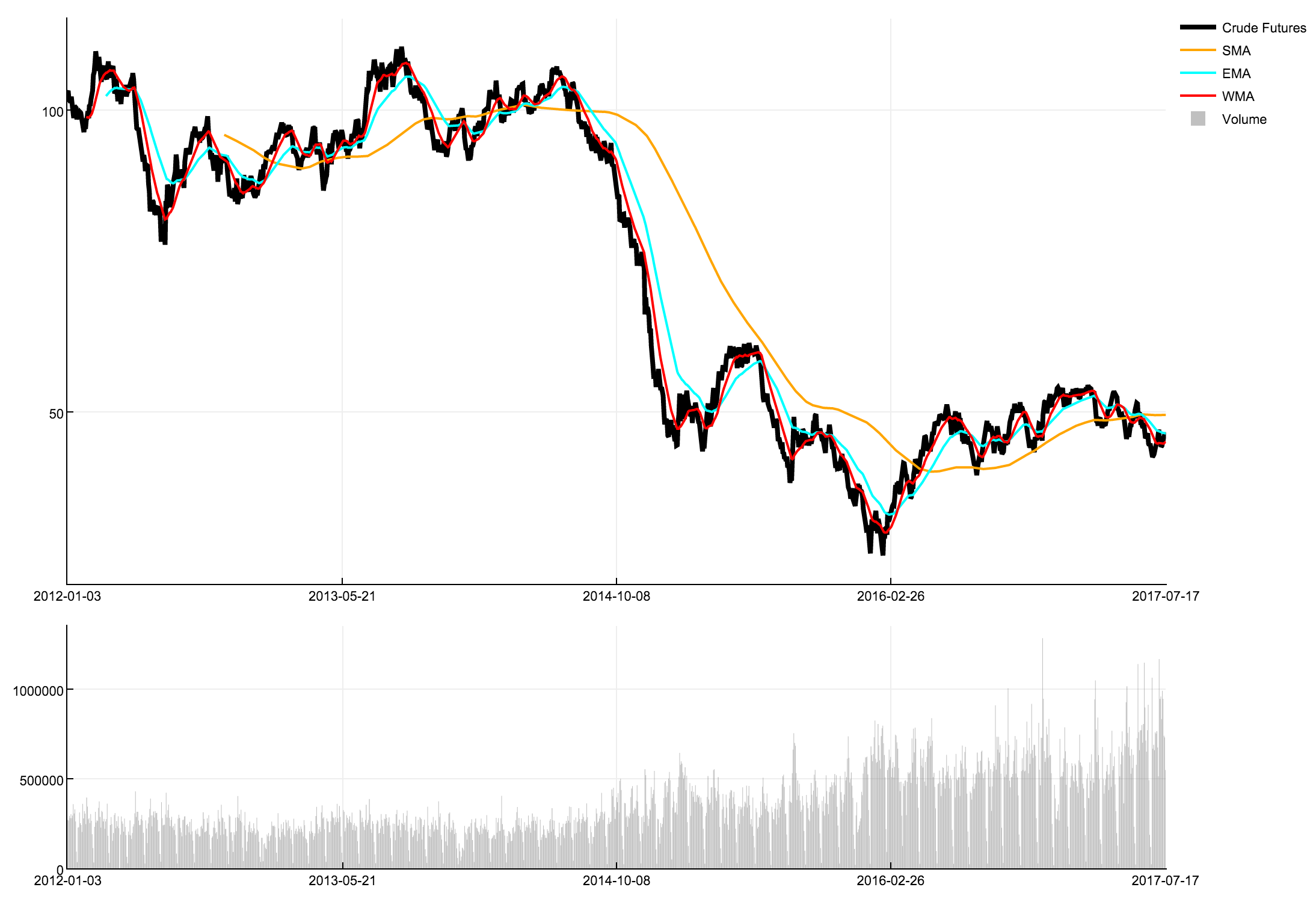
Miscellany
Acknowledgements
This package is inspired mostly by R's xts package and Python's pandas package. Both packages expedite the often tedious process of acquiring & munging data and provide impressively well-developed and feature-rick toolkits for analysis.
Many thanks also to the developers/contributors to the current Julia TimeSeries, whose code I have referred to countless times as a resource while developing this package.
Temporal vs. TimeSeries
The existing Julia type for representing time series objects is a reasonably reliable and robust solution. However, the motivation for developing Temporal and its flagship TS type was driven by a small number of design decisions and semantics used in TimeSeries that could arguably/subjectively prove inconvenient. A few that stood out as sufficient motivation for a new package are given below.
- A key difference is that Temporal's
TStype is defined to bemutable, whereas the TimeSeriesTimeArraytype is defined to beimmutable- Since in Julia, an object of
immutabletype "is passed around (both in assignment statements and in function calls) by copying, whereas a mutable type is passed around by reference" (see here), theTStype can be a more memory-efficient option- This assumes that proper care is taken to modify the object only when desired, a consideration inseparable from pass-by-reference semantics
- Additionally, making the
TSobjectmutableshould provide greater ease & adaptability when modifying the object's fields
- Since in Julia, an object of
- Its indexing functionality operates differently than expected for the
Arraytype, such that theTimeArraycannot be indexed in the same manner- For example, indexing columns must be done with
Strings, requiringArray-like indexing syntax to be done on the underlyingvaluesmember of the object - Additionally, this difference in indexing syntax could cause confusion for newcomers and create unnecessary headaches in basic data munging and indexing tasks
- The syntax is similar to that of the
DataFrameclass in Python. While this a familiar framework, R'sxtsclass is functionally equivalent to the matrix clas - In like fashion, a goal of this package is for the
TStype to behave like anArrayas much as possible, but offer more flexibility when joining/merging through the use of *temporal- indexing, to simplify challenges uniquely associated with managing time series data structures
- For example, indexing columns must be done with
- Another difference between
TSandTimeSerieslies in the existence of a "metadata" holder for the object- While this feature may be useful in some cases, the
TSobject will likely occupy less memory than an equivalentTimeSeriesobject, simply because it does not hold any metadata about the object - In cases where such underlying metadata is of use, there are likely ways to access it without attaching it to the object
- While this feature may be useful in some cases, the
- A deliberate stylistic decision was made in giving Temporal's time series type a compact name
- While the
TimeSeriespackage names its typeTimeArray, typing out nine characters can slow one down when prototyping in the REPL - Creating a type alias is certainly a perfectly acceptable workaround, but only having to type
TS(orts) when constructing the type can save a considerable amount of time if you're experimenting in the REPL for any length of time - Additionally, if you don't want to type out field names every time you instantiate a new time series, the
TSclass will auto-populate field names for you
- While the
So in all, the differences between the two classes are relatively stylistic, but over time will hopefully increase efficiency both when writing and running code.